
| For A-level students |
What is a Matrix?
In mathematics, a matrix is a rectangular array of numbers, symbols, or expressions arranged in rows and columns. It is a fundamental concept used in various fields of mathematics, such as linear algebra, statistics, computer graphics, and more
Types of Matrices
There are quite a few different types of matrices which all have very different uses, today we will be going through some of the more basic structures.
A square matrix is a matrix with the same row and column length. 1×1, 2×2, 3×3, 4×4.
An identity matrix is a square matrix with 1’s down the main diagonal, (top left down to bottom right).
A transposed matrix is a matrix where the rows and columns are swapped around.
A diagonal matrix is a square matrix with only numbers down the main diagonal. A similar matrix is a scalar matrix. The only difference is that the numbers must all be the same.
A triangle matrix is a matrix where all the non 0’s are on one side of the main diagonal.
The two more matrices are the null matrix and the symmetrical matrix.
Below, there are some examples of these structures.

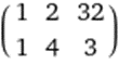
A 2×3 matrix

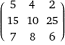
A 3×3 square matrix

A 3×3 Identity matrix

A Transposed matrix

A Diagonal matrix

A Scalar matrix

A Lower Triangular matrix

A Null matrix

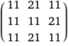
A Symmetrical matrix
Mastering the basic operations on Matrices
Before we begin, some notation must be understood. When referring to a position in a matrix, a coordinate system is used. For example:

The first number corresponds to the row and the second the column so, 1.1 is the first row first column position.
When referring to the size of the matrix we use the notation 2×3, (2 rows 3 columns) and above me is a 3×3 matrix.
Now that this is understood we can move on to the maths.
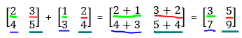
Fortunately, addition and subtraction are very straightforward on matrices. To add matrices, start at the first value, 1.1 (in this case it is the lime undlined 2) and add it to the corresponding value in the matrix being added (also 1.1 which is the lime 1).
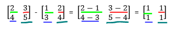
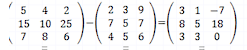
Subtraction is awfully similar. Do the exact same operation but just take away the numbers instead of adding them.
Now it is time to multiply and divide matrices. It should be understood that multiplying by a fraction is the same as dividing. If I asked you to multiply 2 by ½ it is the same as dividing by 2. By using this principle, once you can multiply a matrix, you can divide a matrix.
First, we have to check if two matrices can be multiplied. Two matrices can be multiplied if the number of columns of the first matrix matches the number of rows of the second.
For example, you can multiply a 2×3 with a 3×1 or a 3×2, but you cannot multiply a 2×3 with a 1×3 or a 2×3.

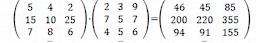
Multiplying matrices is also known as the dot product. In this example we have a 2×3 multiplied by a 3×2.
When multiplying, the first row is multiplied by the first column. This means that we get 1*7, 2*9, 3*11.
7 + 18 + 33 = 58
In notation form, that is 1.1 * 1.1, 1.2 *2.1, 1.3 * 3.1.

This gives us the first value of the new matrix. We repeat this for the next where we multiply the first row by the second column.
Can you finish off the rest?

The Determinant
The determinant tells us the scalar value of the matrix (also known as the magnitude).
The determinant is used to find the inverse of a matrix. When a matrix is multiplied by its inverse, we get the identity matrix.
To calculate the determinant of a 1×1 matrix or 2×2 matrix is easy.
For a 1×1 matrix it is the number in the matrix.
A = [2]
Det(A) = 2
For a 2×2 matrix it is slightly harder.

Det(A) = 6
But why and how do we calculate this?
By multiplying the main diagonal together (yellow) then multiplying the inverse of the main diagonal together and then taking these numbers away from each other.
2*4 = 8
2*1 = 2
8-2 = 6
Therefore, the determinant is 6.
Determinant of a 3×3
By learning how to do the determinant of a 3×3, you can use the same principles to work out the determinant of a 4×4 however, it is unlikely to be asked as computers are very good to doing this for us.
It is important to be able to calculate the determinant of a 3×3 matrix but only understand how to calculate the determinant 4×4.
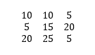
Let us go through the process. Firstly, we need a 3×3 matrix.

Det(A) = 279
How did we get 279?
Firstly, we need to create the minor matrices. These are 2×2 matrices created from the 3×3.
For clarity, we will swap out the first row with letters.


The first minor matrix is the “i” matrix:

We ignore any values in the same row or column therefore, we are left with:

Now we calculate the determinant of this 2×2.
(8*0) – (9*11) = -99
But wait we didn’t include i. Let us replace i with its value, 1. Because 1 is outside the matrix, it multiplies every number of the matrix like normal multiplication. So:
-99*1 = -99
This is our first value. We have to do the same for j and k.

-j[(6*0) – (0*11)] = j*0
j = 5
-5*0 = 0
And now k

k = 7
7[(6*9) – (0*8)] = 11*54
7*54 = 378
The determinant is all these values added together.
Det(A) = -99 -0 + 378 = 279
Did you notice that for j, a minus was put in front of the equation. This is part of the process. To make it clearer, here is a matrix showing what sign to put in front of the minor matrix.

Since i, j and k where on the top row we use that.
i has a plus so nothing changes as does k.
So only j has to swap signs.
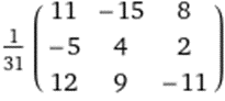
Try finding the determinant of:
Answer: -1375
Inverse
To work out the inverse of a matrix, there are multiple methods. The method we will use is called the Gaussian elimination method. This is better than the traditional a-level method because we can use it for LU decomposition and eigen vectors/values so pay attention!
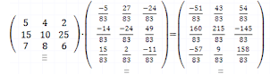
Let us start with a simple example:

Using the mathematical principle that a matrix multiplied by its inverse is equal to the identity matrix, we can solve this.

By changing matrix A into the identity matrix, we have the steps to change the identity matrix into the inverse of A. By completing this example, it will become much clearer.
There are only 3 operations that can be done to the matrix. These are, swapping the rows around (R1, row 1 swaps with R3, row 3), multiplying a row by a number and adding/subtracting a row from another (R1 – R3, row 1 minus row 3, in the example that would leave [0,0,-1]).
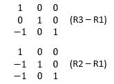
Firstly, let’s make the A matrix into the identity matrix and record the steps.

This is a very simple example, but it is the same method for all matrices.
Now we apply these steps to the identity matrix.
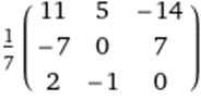
And there we have it. That is how you find the inverse. Try it on this matrix:

Answer:

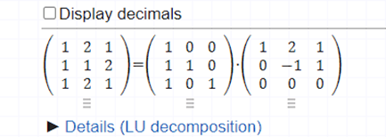
LU Decomposition
Lower and Upper matrix decomposition is a way to represent 1 matrix as 2.
How do we do it?
Let’s take this matrix:

A can be represented as A = [L][U]
To get L and U we use Gaussian elimination to calculate U and save the steps we took to get L.
Lets create L alongside the original matrix so we can save the steps.
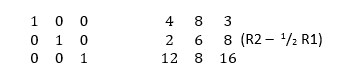
Every step we do to the right hand matrix, we do to the left hand matrix.

For the L matrix, we swap the signs around and there we have it.

The LU decompositions is finished.
Eigenvectors and Eigenvalues
This will be the last tutorial on this sheet. This is by far the hardest and most confusing bit. We will start with Eigenvalues as these lead to Eigenvectors.
This will be easier than a question given as we will only be looking at how to calculate these values and not why we use them and how to manipulate equations into the form needed to use Eigenvectors.
To get the Eigenvalues is quite simple.

Det(A-I*λ) = 0
What this equation means is that by multiplying the identity matrix by lambda and taking it away from A, the determinant of this matrix is 0. This leads to forming a cubic equation to be solved (quadratic for a 2 by 2).

Now we need to calculate the determinant of this matrix.


When we combine these answers of the minor matrices, we get:
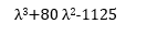
Remember that, Det(A-I*λ) = 0 therefore,

Solve the cubic!

These are the Eigenvalues! This worksheet is just to show you how to get them, but we recommend you looking up their uses in the real world.
Now let us get the Eigenvectors from these values.
Bx = 0
Where x is an Eigenvector and B is the A-I*λ matrix because
(A-I*λ)*x = 0
Calculating the first Eigenvector using
Now we have B so now we have to work out x.
We can start by partitioning the matrix.

To solve this, we need to reduce the matrix to an Upper matrix. (It may help to think of this as an algebraic equation, Column 1 is x1 Column 2 is x2 and Column 3 is x3. -69.823 x1 + 5 x2 + 15 x3 = 0 and to solve an equation we need to work out the value of the variables and we do this by creating an Upper matrix).

From this matrix we can get the equations
-69.823 x1 + 5 x2 + 15 x3 = 0
-53.391 x2 + 34.297 x3 = 0
0 x3 = 0
This last equation is also known as a free parameter (free because it can be any number we want) so:
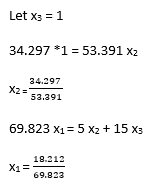
Now we have the values of the Eigenvector lets build it up

where x1 = 0.261, x2 = 0.642 and x3 = 1
That is the Eigenvector for the Eigenvalue 79.823. This is then repeated to calculate the other 2 Eigenvectors. Which are:

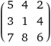
This was quite a hard example! However, it does show how you can do it. How about you try this matrix! Find the 3 Eigenvalues and their Eigenvectors.

Video with explanation on how to do it
This video solves the above problem and teaches Eigenvalues and Eigenvectors if you still do not understand
Exercise 1.1
What type of matrix is it?
1)

2)

3)

4)

5)

6)

Exercise 1.2
Adding and subtracting
+

=

+

=

–

=
Exercise 1.3
Multiply and divide matrices

*

=
/

=
(hint make second matrix inverse)

*

=

*
=
Exercise 1.4
Find the determinant


Exercise 1.5
Find the inverse


Exercise 1.6
LU decomposition


Exercise 1.7
Eigenvalues + Eigenvectors


Answers:
1.1
3×3 matrix
diagonal matrix + scalar matrix
identity matrix
upper matrix
lower matrix
symmetrical matrix
1.2


1.3


1.4
7
559
-121,856
1.5


1.6


1.7


